How to Add Power Pivot to Excel & Access the Data Model

Power Pivot is a powerful tool within Excel for storing, analysing, and calculating large amounts of data – even millions of rows - using relational data models. It allows you to go beyond Excel’s traditional two-dimensional spreadsheet format and instead work with data using a robust structured approach, optimised for speed and scale.

You can import data into Power Pivot from many different sources using the Power Query tool, and then create calculated columns and measures with DAX (Data Analysis Expressions). From there, you can create:

• PivotTables to quickly slice and dice the data
• Financial statements, reports and dashboards in an Excel worksheet using CUBE functions that filter and aggregate the Data Model.

If you don’t see Power Pivot in your Excel Ribbon by default, you’ll need to enable it.

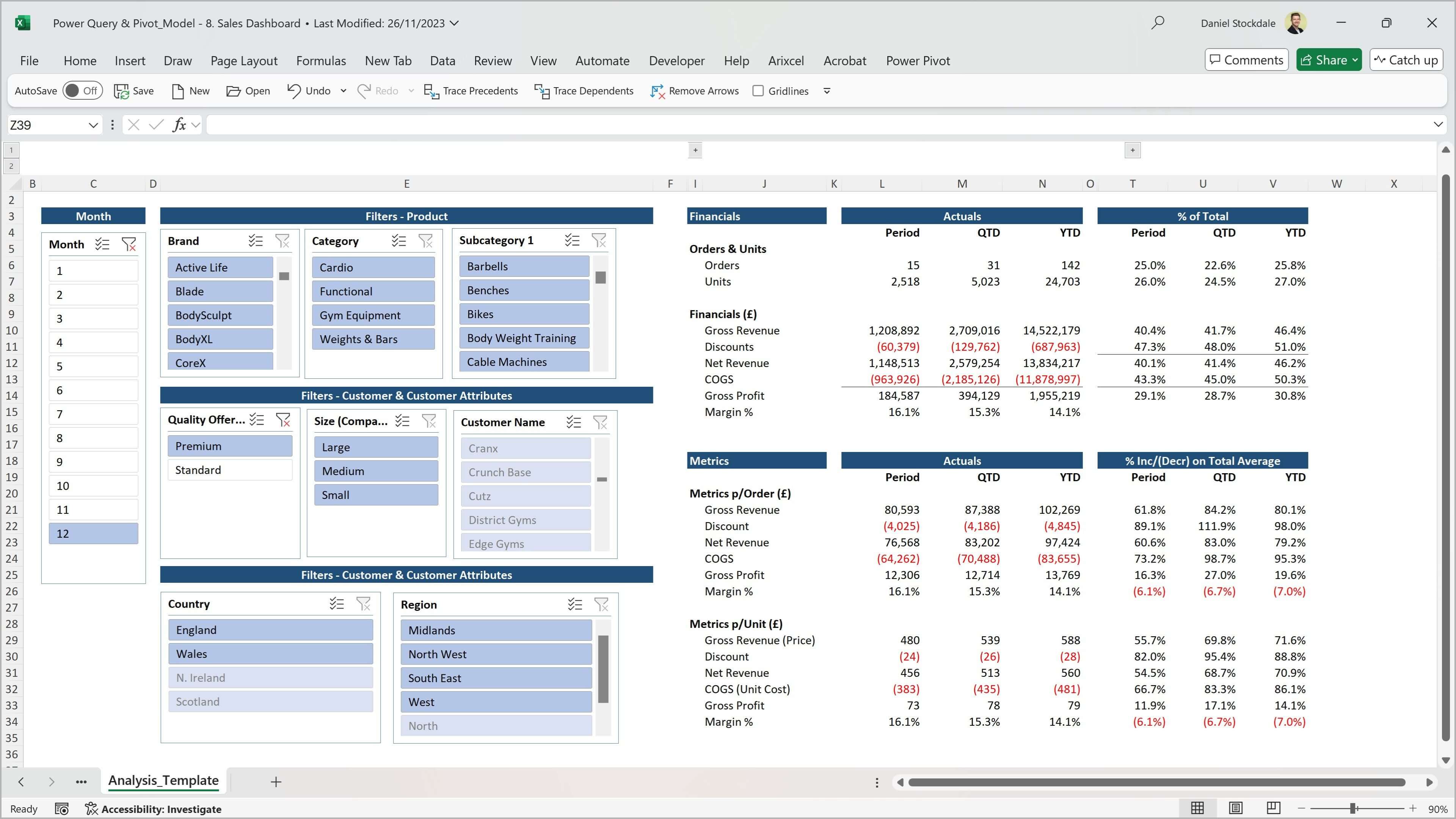
Sales Dashboard in Excel worksheet filtering and aggregating a Power Pivot data model. Note: Power Pivot tab is visible at top-right of Ribbon.

Adding Power Pivot to the Ribbon

1. Go to File > Options.
2. Select Add-ins from the left-hand menu.
3. At the bottom, in the Manage drop-down, choose COM Add-ins and click Go.
4. Tick the box for Microsoft Power Pivot for Excel and click OK.

You should now see a Power Pivot tab in your Ribbon.

Tick the Microsoft Power Pivot for Excel option in the COM Add-ins dialog box to enable Power Pivot.

Accessing the Power Pivot Window and Data Model

Once the Power Pivot add-in is enabled, you can start creating the Data Model and working with imported tables of data. This all takes place in the Power Pivot Window. There are two ways to access it:

1. Via the Power Pivot Ribbon:
• Click on the Power Pivot tab.
• Select Manage. This opens the Power Pivot window, where you’ll see all tables in the model.
2. Via the Data Ribbon:
• Go to the Data tab.
• In the Data Tools group, click Manage Data Model (a small green icon).

Both routes take you to the same place - the Power Pivot window.

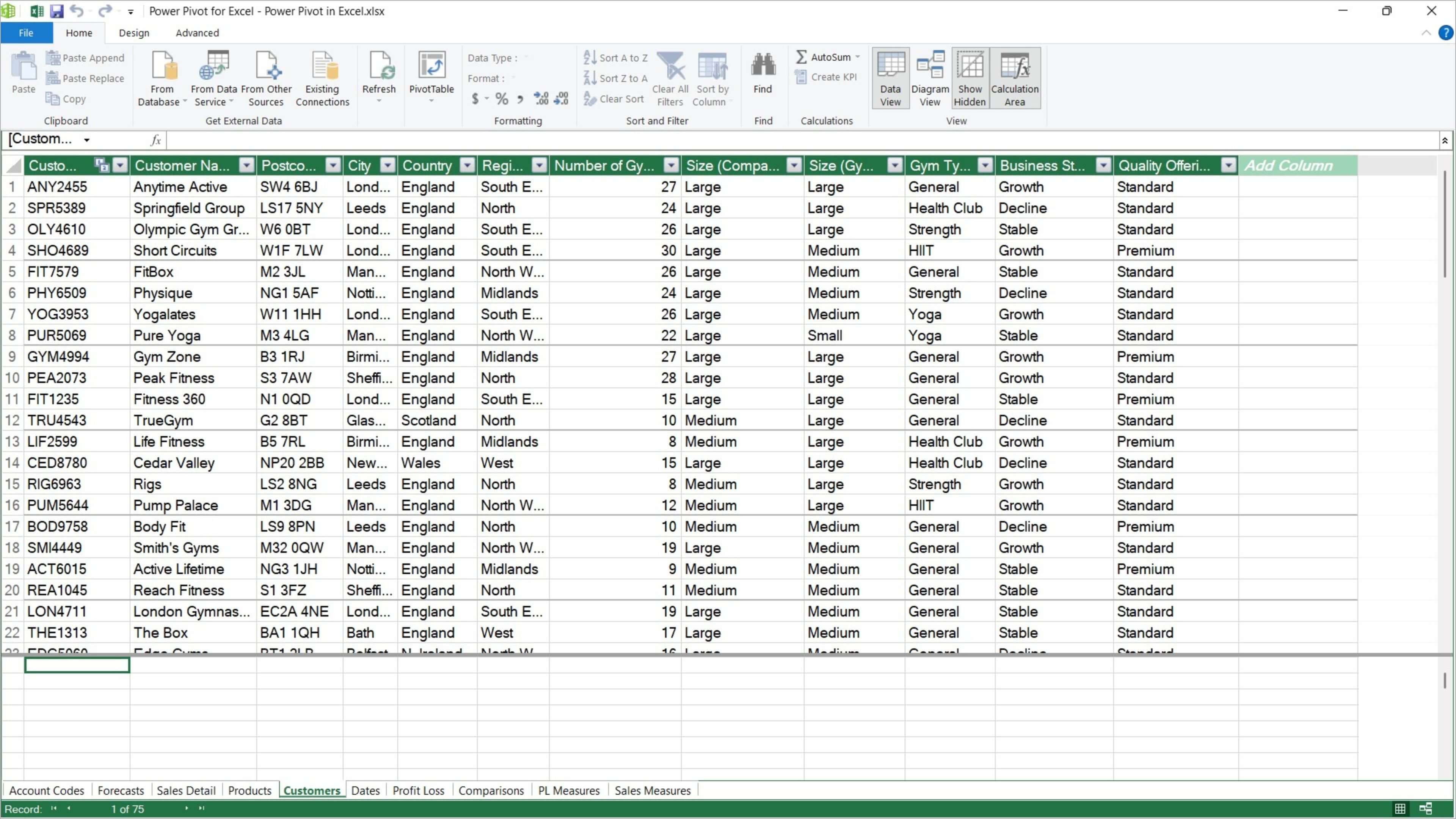
Power Pivot window showing imported data in Data View.

Data View and Diagram View

Inside the Power Pivot window, go to the Home tab to switch between two views in the View group:

• Data View: Displays tables of data imported into Power Pivot in a grid format, similar to Excel worksheets. This is where you can inspect imported data, add calculated columns, or check data types.
• Diagram View: Displays tables of imported data as boxes and lists their column names. Here you can build the Data Model by dragging and dropping fields between the tables to create relationships.

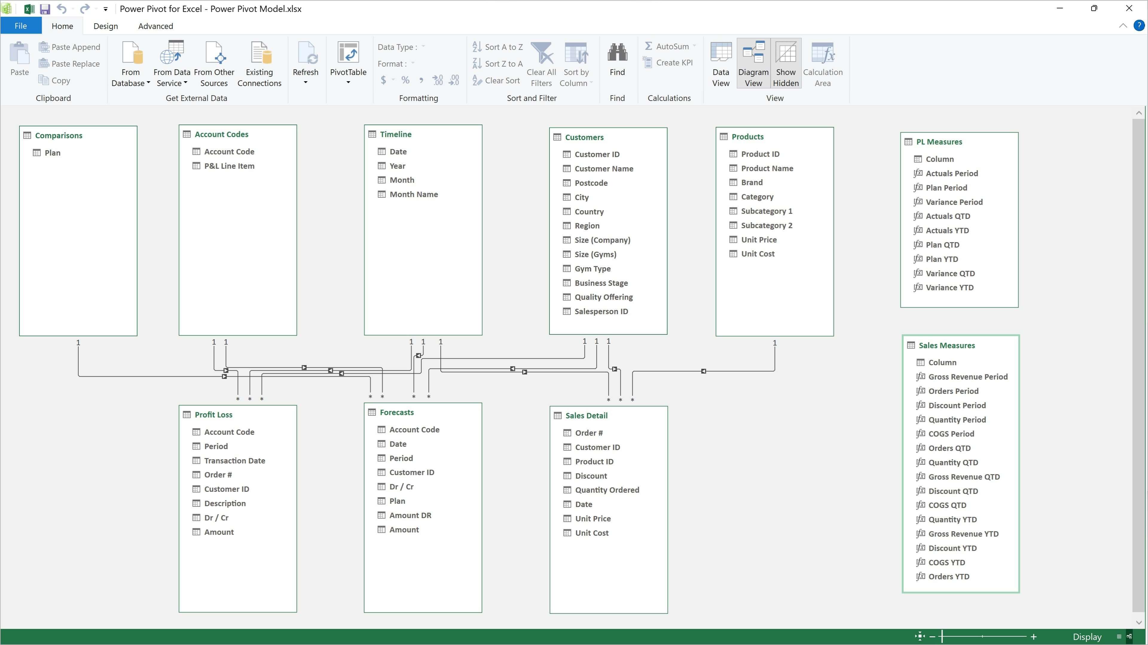
Power Pivot window showing the Data Model in Diagram View.

How to Learn More

By enabling Power Pivot and learning how to create and leverage the Data Model, you unlock a whole new level of analysis in Excel. Our course Power Query & Power Pivot: Automating Reporting teaches you how to leverage more of your organisation’s data, automate workflows to save time, and build highly responsive financial reports.